In my last post, I compared Jev with two custom models built from labeled comments: a small neural network (MLP) and k-nearest neighbors (k-NN). Both custom models start from an embedding of each comment, and with cloud embeddings they beat Jev once they had about a hundred labels.
Another common way to build a text classifier is to fine-tune a pretrained language model like BERT, and I was curious how that would perform against Jev. It works differently from the custom models in the last post. In both of them, an embedding model turns each comment into a list of numbers once, and that list never changes. The MLP can only learn which of those numbers matter, not how to compute better ones. Fine-tuning adjusts every one of the language model's weights on the labeled data instead.
So I fine-tuned BERT on the same 8,000 comments and scored it on the same 2,000. The short version: on the common labels, it's the best model in the comparison, and nothing goes to the cloud. But it's slower, much bigger, and it misses almost every comment on the two rarest labels.
Fine-tuning vs. frozen embeddings. In the last post, the embedding model was a fixed first step: it read the comment and produced a list of numbers, and the MLP only ever saw those numbers. Fine-tuning removes that boundary. A small classification layer goes on top of the language model, and training updates the whole stack, so the model can learn to pay attention to the words and phrases that matter for toxicity, like tone, slurs or a "you" aimed at another person, instead of whatever the embedding model was originally trained to capture.
The setup
Everything that was in the last post stays the same: the first 10,000 comments from the Jigsaw Toxic Comment Classification Challenge, the same 8,000 for training and 2,000 for evaluation, the same six labels and the same metrics. The other approaches' numbers are unchanged.
The new model is bert-base-uncased, a 110-million-parameter model from 2018, with one output for each of the six labels. I trained it once with a standard recipe: 3 passes over the 8,000 comments, a learning rate of 2e-5, batches of 16, and each comment cut to its first 128 tokens. I didn't tune any of these on the evaluation set, or at all. Training took 9 minutes on the GPU of an Apple M1 Pro laptop.
The core of the training loop is short, using the Hugging Face transformers library:
model = AutoModelForSequenceClassification.from_pretrained(
    "bert-base-uncased",
    num_labels=6,
    problem_type="multi_label_classification",
)
optimizer = torch.optim.AdamW(model.parameters(), lr=2e-5, weight_decay=0.01)
loss_fn = nn.BCEWithLogitsLoss()

for batch, labels in batches:
    loss = loss_fn(model(**batch).logits, labels)
    loss.backward()
    optimizer.step()
    scheduler.step()
    optimizer.zero_grad()
The difference from the last post is in the optimizer line. With frozen embeddings, the optimizer only gets the MLP's weights. Here it gets model.parameters(), all 110 million of them. The full script, with batching and evaluation, is src/eval_bert.py in the repository.
Ranking comments
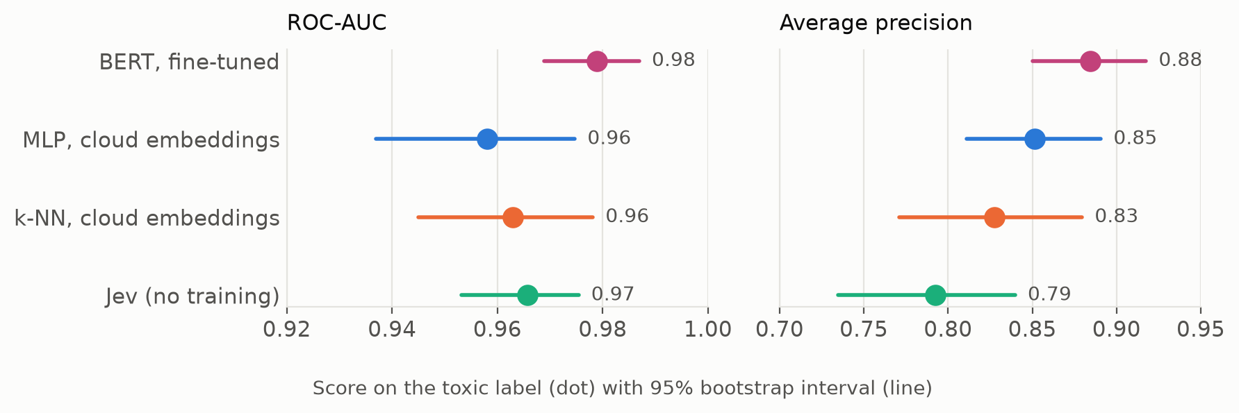 Figure 1: How well each approach ranks toxic comments above clean ones on the
 toxic label. Each line is a 95% bootstrap interval. Fine-tuned BERT has the best score on both.
On toxic, BERT reaches 0.98 ROC-AUC and 0.88 average precision, the best of the four on both. The gap to the MLP on cloud embeddings, 0.88 against 0.85, is small but holds up: in a paired bootstrap, BERT comes out ahead in 99% of resamples. Against Jev, it's ahead in every resample.
ROC-AUC hides where the models differ, because all four curves crowd into the top-left corner. Zooming into that corner, where only a small share of clean comments get flagged, makes the differences visible:
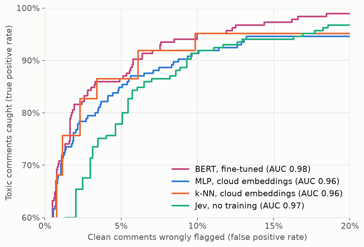 Figure 2: The top-left corner of the ROC curve on
 toxic. Each curve shows the share of toxic comments caught (up) against the share of clean comments wrongly flagged (right). Higher is better.
If you accept flagging 2% of clean comments, about 36 of the 1,815, BERT catches 82% of the toxic ones. The two cloud models catch about 76%, and Jev catches 60%. Jev only catches up with the MLP when about 10% of clean comments get flagged. That's why Jev's ROC-AUC (0.97) is higher than the MLP's (0.96) while its average precision is clearly lower: Jev does well in the part of the curve that matters least in practice. The k-NN curve moves in big steps because, with 7 neighbors, it can only give 8 different scores.
It isn't the best ranker I've built on this dataset, though. In the last post, k-NN on cloud embeddings with 51 neighbors reached 0.90 average precision. BERT and that k-NN are a statistical tie.
Making decisions
The scores are also well calibrated. BERT's default 0.5 threshold gives 0.81 F1 on toxic: it catches 146 of the 185 toxic comments and flags 30 clean ones. With a threshold picked fairly, the same way as in the last post, the best threshold lands at 0.44, right next to the default.
| Approach | toxic F1 with a fair threshold | Average F1, all six labels |
|---|---|---|
| BERT, fine-tuned | 0.80 | 0.49 |
| k-NN, cloud embeddings | 0.80 | 0.57 |
| MLP, cloud embeddings | 0.77 | 0.54 |
| Jev | 0.70 | 0.51 |
On toxic, BERT ties k-NN on cloud embeddings for the best F1. Better ranking doesn't always become better decisions, which is what I saw with 51-neighbor k-NN too. Averaged over all six labels, in the right-hand column, BERT drops below Jev, because of the two rarest labels.
The rare labels
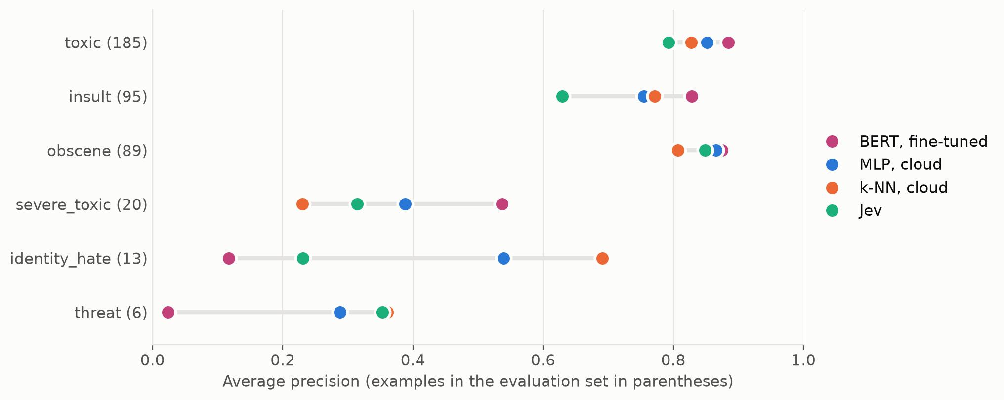 Figure 3: Average precision on each label, with the number of examples in the evaluation set in parentheses. BERT leads on the four larger labels and scores close to zero on the two smallest.
On the four labels with at least 80 training examples, BERT is first or tied for first on average precision:
| Label (training examples) | BERT | MLP, cloud | k-NN, cloud | Jev |
|---|---|---|---|---|
toxic (786) | 0.88 | 0.85 | 0.83 | 0.79 |
obscene (438) | 0.87 | 0.87 | 0.81 | 0.85 |
insult (399) | 0.83 | 0.75 | 0.77 | 0.63 |
severe_toxic (81) | 0.54 | 0.39 | 0.23 | 0.32 |
BERT's biggest lead is on insult. In the last post, Jev trailed there because the raters used the label more narrowly than my question did. BERT learned that narrower definition better than any other model, though with a fair threshold, k-NN still edges it on F1, 0.73 against 0.71.
Then there are threat and identity_hate, with 27 and 71 training examples. BERT doesn't learn to find either of them. Across all 2,000 evaluation comments, its highest threat score is 0.23, so at any sensible threshold it never flags a threat. The six real threats score 0.09 or lower, and the median one ranks around 120th. Its average precision on identity_hate is 0.12, against 0.54 for the MLP on cloud embeddings.
The likely explanation is that all six labels share one model, trained together for three short passes. With 27 threats among 8,000 comments, they barely move the training loss, and the model spends its effort on the common labels. The cloud-embedding models don't have this problem to the same degree: the embedding already puts threats close together, so even a handful of examples is enough to find them. Weighting the rare labels more heavily, training longer, or training a separate model per label would probably help, but I haven't tested that.
How many labels does it need?
The last post's most useful chart showed how quality changes with the number of labels. I repeated it for BERT, training on 50 to 1,000 comments, three times per size, with the same random subsets the MLP and k-NN used. Each run got 1,500 training steps, the same as the full 8,000-comment run, so a small training set is seen many more times. That's the same rule the MLP sweep follows, and it matters. My first sweep gave the small runs only 200 steps, and 4 of its 15 models didn't catch a single toxic comment at the default 0.5 threshold.
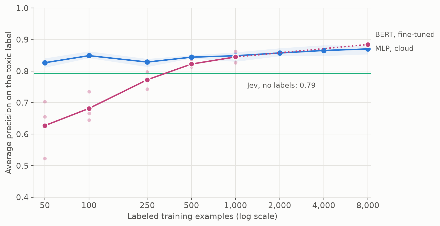 Figure 4: Average precision on
 toxic as the training set grows. Light dots are individual BERT runs, and the MLP line is the average over the same three subsets. The dotted segment joins the sweep to the single full-data run, with no runs in between.
| Labeled comments | BERT | MLP, cloud | Jev |
|---|---|---|---|
| 50 | 0.63 | 0.83 | 0.79 |
| 100 | 0.68 | 0.85 | 0.79 |
| 250 | 0.77 | 0.83 | 0.79 |
| 500 | 0.82 | 0.84 | 0.79 |
| 1,000 | 0.85 | 0.85 | 0.79 |
| 8,000 | 0.88 | 0.87 | 0.79 |
Average precision on toxic, averaged over the same three training subsets. The 8,000 row for BERT is the single full run. Jev uses no labels, so its score doesn't change. The MLP's 8,000 row comes from the sweep, which trains it a little differently from the single run in Figure 1, so it reads 0.87 here instead of 0.85.
- Fine-tuning needs labels to make up for the embedding. The cloud embeddings are already good at toxicity before the MLP sees a single label, so the MLP is near its best from 50 comments. BERT has to learn it, and only catches up at around 1,000 labels.
- It passes Jev at around 500 labels on
toxic. All three runs at 500 beat Jev's 0.79, and at 250 only one of them did.
The default threshold doesn't hold up on small training sets. At 50 labels, BERT's average F1 at 0.5 is 0.31, against 0.69 for the MLP on cloud embeddings. Small runs rank comments better than their F1 suggests, but their scores sit in the wrong place, so they'd need a threshold picked on held-out labels, the way Jev's threshold was picked in the last post.
Averaged over all six labels, BERT trained on 1,000 comments reaches 0.53 average precision. That's about as good as with all 8,000 and better than the MLP on cloud embeddings with the same 1,000. The 1,000-comment runs went through their data 24 times, against 3 times for the full run. That's a hint that the full run's failure on threat and identity_hate comes from too little training, not too little data, but I haven't tested it directly.
Speed, size and cost
| Model | Median time per comment | Size | Where the comment goes |
|---|---|---|---|
| BERT, laptop CPU | 52 ms | 438 MB | Nowhere |
| BERT, Apple M1 Pro GPU | 13 ms | 438 MB | Nowhere |
| Cloud embeddings + MLP | 254 ms | 2 MB | |
| Jev, all six questions | 209 ms | none | TypeSafe |
I timed BERT on the same AMD Ryzen 7 5800H CPU as the local pipelines in the last post, one comment at a time with four threads, and on the GPU of an M1 Pro. Even on the CPU, it's four times faster than a round trip to either cloud service. It costs nothing per comment.
The costs are elsewhere:
- Training needs a GPU. Fine-tuning on 8,000 comments took 9 minutes on the M1 Pro's GPU. On the Ryzen's CPU, fine-tuning on just 100 comments, for 200 training steps, took about 9 minutes. The MLP from the last post trains on all 8,000 comments in 3 to 7 seconds.
- It's big. At 438 MB, running it in a reader's browser, as I did with a smaller model in an earlier post, would mean a large download.
- It's one model per definition. With frozen embeddings, changing a label means retraining a small MLP in seconds, or nothing at all for k-NN. With fine-tuning, any change to the labels means fine-tuning the whole model again.
What this doesn't tell you
- It's one training run. The full-data numbers come from a single run with one random seed and an untuned, standard recipe. Another seed would move them a little, and tuning would probably help, especially on the rare labels.
- The label sweep has fewer repeats. Each training size was repeated three times for BERT, against ten for the MLP and k-NN, because each BERT run takes minutes instead of seconds.
- The labels are still noisy. Of the 37 clean-labeled comments that Jev was most confident were toxic, many of them plainly hostile, BERT flags 16. The MLP on cloud embeddings flags 14. Models trained on these labels learn the raters' habits, including their mistakes.
Conclusion
The last post ended with "the first thing to get right is the embedding model". Fine-tuning adds a second answer: let the model learn its own representation. A fine-tuned BERT running on my own hardware ranked toxic comments better than anything built on cloud embeddings, except a k-NN it tied, and its default threshold worked without tuning. Nothing leaves the machine.
But it needs a GPU to train, it's a 438 MB model, and on the rarest labels it did worse than Jev, which never saw a single example. For the common labels, with thousands of examples and a GPU, fine-tuning is the strongest option I've tried. For my blog, with a hundred comments and one question, it doesn't change my choice: Jev is still the right trade.
What to try next
- Fix the rare labels. The label sweep hints that the full run simply didn't train long enough on
threatandidentity_hate. Training for more passes, weighting the rare labels more heavily in the loss, or training a separate model per label are all small changes to the loop above. - Fine-tune a smaller model. A smaller model like DistilBERT could keep most of the quality at a size that fits in a browser.
The code, cached predictions and analysis scripts are in the repository, including the sweep script, so you can try either one yourself. If you do, I'd love to hear how it goes!
Comments
No comments yet. Be the first to comment!
Leave a comment
Comments are moderated and may take some time to appear.