
In my last post, I skipped training a comment spam filter for this blog and used Jev, TypeSafe's "System One" decision model, instead. I described what spam looks like in plain language, asked Jev a yes/no question (Noul) for each comment, and got a 0.922 ROC-AUC without collecting a single training example.
I ended that post with a question I couldn't answer:
I didn't build the custom model, so I can't say how Jev compares to one. A model trained on my own comments might well be more accurate.
The blog still has around a hundred comments, which isn't enough to train anything. But I've trained this kind of model before. In an earlier post, I built a toxicity classifier for the Jigsaw Toxic Comment Classification Challenge dataset: generate an embedding for each comment, then train a small PyTorch network on top of the embeddings. That gives me labeled data, a training pipeline, and a model I already know how to build. So I ran Jev on the same comments and compared.
The short version: a custom model does beat Jev, but by less than I expected, and it needs fewer labels to get there than I expected too. The choice of embedding model turned out to matter more than anything else in the comparison.
The setup
The dataset is the first 10,000 comments from the Jigsaw training set, which are Wikipedia talk page comments labeled by human raters. Each comment has six yes/no labels: toxic, severe_toxic, obscene, threat, insult and identity_hate. A comment can have any number of them. I split the comments into 8,000 for training and 2,000 for evaluation, and every number in this post comes from those same 2,000 comments.
Toxic comments are rare, and some labels are very rare:
| Label | Positives in the 2,000 evaluation comments |
|---|---|
toxic | 185 (9.3%) |
insult | 95 (4.8%) |
obscene | 89 (4.5%) |
severe_toxic | 20 (1.0%) |
identity_hate | 13 (0.7%) |
threat | 6 (0.3%) |
Most of the numbers in this post are for toxic. It's the broadest label, the closest to the single yes/no question in my spam filter, and with 185 examples it's the only one large enough to measure precisely. I come back to the other labels later.
In the original post, I reported that the model reached 98% accuracy. That number is less impressive than it sounds: since 96.6% of all the labels in the evaluation set are "no", a model that always answers "no" gets 96.6% accuracy while catching nothing. This post uses metrics that only reward finding the toxic comments.
I compared three approaches:
- A small neural network, a multilayer perceptron (MLP), trained on the 8,000 labeled comments. It's the same model from the earlier post.
- k-nearest neighbors (k-NN), which doesn't train at all. It classifies a comment by looking at the 7 most similar labeled comments.
- Jev, which never sees the training data. Each comment is sent with six Noul questions, one per label, and Jev returns six probabilities. The questions follow the same pattern as the spam filter: an instruction plus a description of what counts as "yes" and as "no". For example,
toxicis "rude, disrespectful, hostile, abusive, profane, insulting, threatening, or hateful language directed at another person or group", while civil disagreement and criticism of an edit is not. The full text of all six questions is in the repository.
If you haven't worked with these before, here's how the MLP and k-NN work. Both start from embeddings. An embedding model turns a piece of text into a list of numbers, called a vector, so that texts with similar meanings get similar vectors. You can picture each comment as a point in space, where nearby points are comments that say similar things.
- k-NN uses that space directly. To classify a new comment, it finds the k labeled comments closest to it and lets them vote. With 7 neighbors, if 4 of them are labeled toxic, the new comment gets a toxic score of 4/7, or 0.57. There's no training step: the labeled comments are the model.
- An MLP is the simplest kind of neural network: a few layers that each combine the numbers coming in using a set of weights, apply a simple function, and pass the result on to the next layer. Training shows it the embeddings of the labeled comments over and over, adjusting the weights a little each time until its outputs match the labels. Once trained, it only needs those weights, not the labeled comments, and it can learn which parts of the embedding matter for the task.
The MLP and k-NN both need an embedding for each comment, so I tried each of them with two embedding models:
- Cloud embeddings: Google's
gemini-embedding-001with theCLASSIFICATIONtask type, truncated to 768 dimensions, or 768 numbers per comment. This is an API call per comment. - MiniLM embeddings:
all-MiniLM-L6-v2, a small model that produces 384 numbers per comment and runs locally, even in the browser. It's the model from the earlier post.
That's five configurations: the MLP and k-NN on each embedding model, plus Jev.
In the rest of this post, I'll call the MLP and k-NN the custom models. Only the MLP is trained, but both are built from the labeled comments, while Jev only gets my questions.
Ranking comments: a tie that isn't quite a tie
The first question is whether each approach scores toxic comments higher than clean ones. That doesn't need a threshold, so it's the fairest comparison to start with.
Two metrics describe how well a classifier ranks:
- ROC-AUC is the chance that a random toxic comment scores higher than a random clean one. Here, a random guess scores 0.5.
- Average precision measures how clean the top of the ranking is: if you go down the list from the highest score, how many of the comments you pass are actually toxic? Here, a random guess scores 0.09, the share of toxic comments.
When positives are rare, ROC-AUC can look great even when the top of the list is full of mistakes, because there are so many clean comments to rank below. Average precision doesn't hide that.
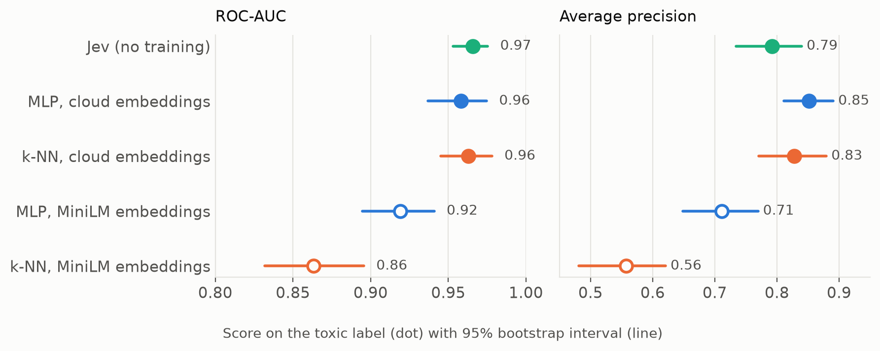 Figure 1: How well each approach ranks toxic comments above clean ones on the
 toxic label. Each line is a 95% bootstrap interval. Jev ties the custom models built on cloud embeddings on ROC-AUC, but trails them on average precision.
On ROC-AUC, Jev scores 0.97 and both models trained on cloud embeddings score 0.96. The differences are well inside the intervals, so this is a three-way tie. That's still remarkable for a model that has never seen this dataset.
Average precision tells a different story. The MLP on cloud embeddings reaches 0.85, k-NN 0.83, and Jev 0.79. The gap between Jev and the MLP is real: in a paired bootstrap, the MLP comes out ahead in more than 99% of resamples. Both custom models put fewer clean comments among their most confident predictions.
Both models on MiniLM embeddings trail Jev on every metric, by a wide margin.
A probability isn't a decision
Ranking is only half the job. To act on a comment, I need a threshold, and that's where the first surprise from the spam post shows up again.
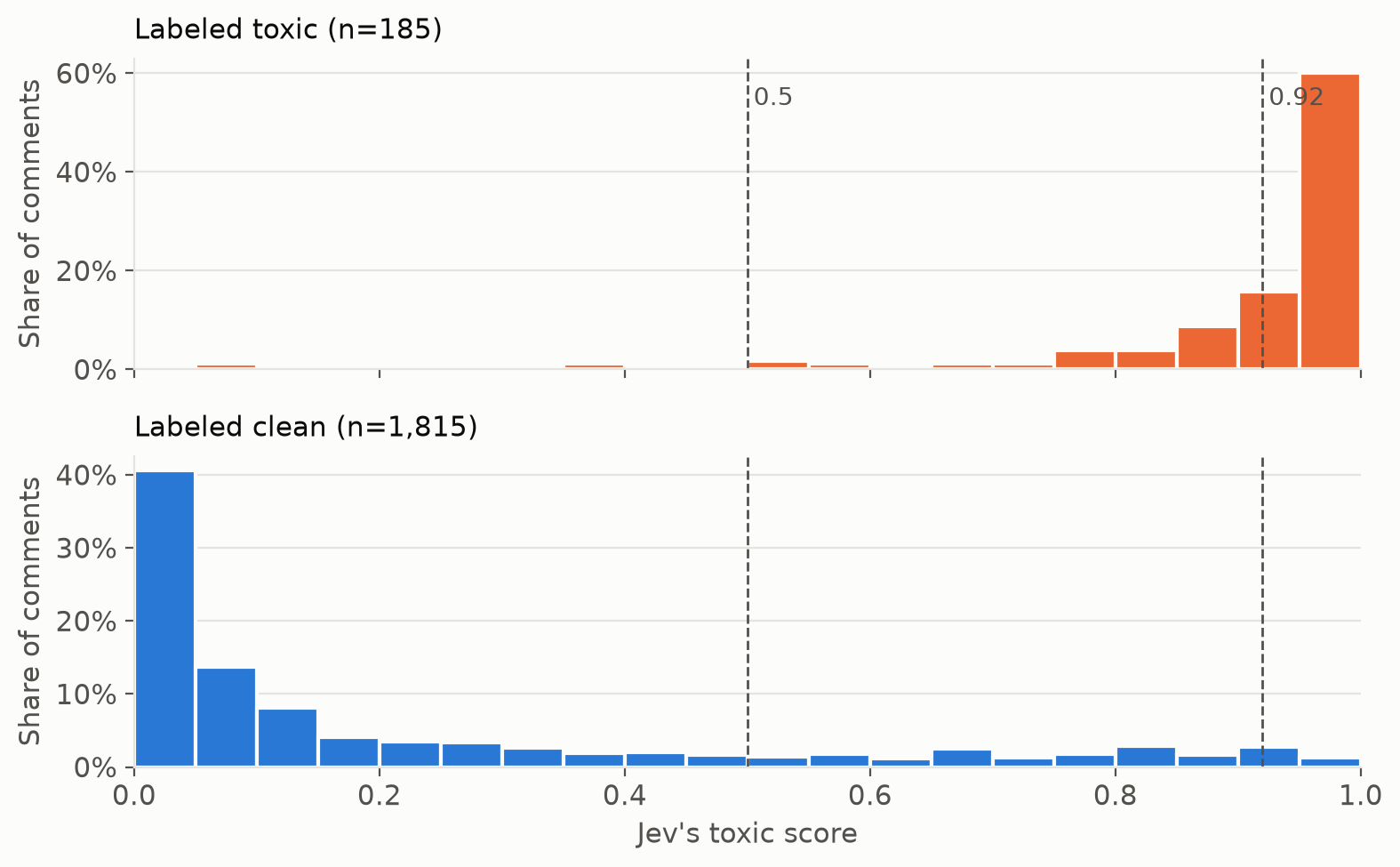 Figure 2: Jev's
 toxic score for every evaluation comment, split by how the raters labeled it. Toxic comments pile up near 1.0, while clean comments have a long, thin tail that reaches all the way up.
That tail is the problem. Most clean comments score close to 0, but there are so many of them that even a thin tail adds up to hundreds of comments above 0.5.
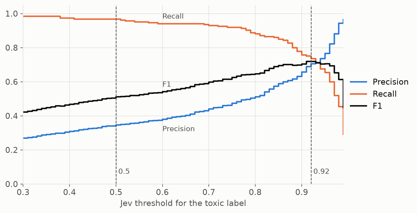 Figure 3: Jev's precision, recall and F1 on the
 toxic label as the threshold changes. At the default 0.5, it catches 97% of toxic comments, but only 35% of what it flags is labeled toxic. F1 peaks around 0.92.
| Threshold | Toxic flagged (of 185) | Clean flagged (of 1,815) | Precision | Recall | F1 |
|---|---|---|---|---|---|
| 0.5 | 179 | 337 | 0.35 | 0.97 | 0.51 |
| 0.8 | 163 | 156 | 0.51 | 0.88 | 0.65 |
| 0.9 | 140 | 73 | 0.66 | 0.76 | 0.70 |
| 0.95 | 121 | 37 | 0.77 | 0.65 | 0.71 |
| 0.98 | 84 | 5 | 0.94 | 0.45 | 0.61 |
At 0.5, Jev flags 337 comments the raters labeled as clean. The custom models don't have this problem: their scores come from the labels, so they already reflect how rare toxicity is in this dataset and how strict the raters were, and their 0.5 sits in a sensible place. Jev only knows what my question says.
I wanted to know whether those 337 comments were Jev being wrong or Jev being stricter than the raters, so I read the 37 that Jev was most confident about, all scoring 0.95 or higher. By my count, about two-thirds of them are plainly hostile. A few examples, all labeled clean:
- "OMG, you are an imbecile."
- "You are clearly not very smart and not here to build an encyclopedia."
- "Stay off my talk page, stalker."
- A message telling an administrator it "is not difficult to learn precisely who in that real world the coward is behind the loud account", which reads as a veiled threat.
Five of the 37 have one of the other labels, such as insult, but not toxic, so the dataset contradicts itself on those. The rest are mostly heated arguments that could go either way, plus a few real mistakes, like a polite request to unblock a user. On the other side, the toxic-labeled comments Jev scored lowest include a barnstar thanking an editor for fighting vandalism, and a suggestion to add a "Mobile porn" link to an article.
Precision measured against human labels caps out at how consistent those labels are. A model built from labels learns the raters' habits, including their mistakes. Jev applies the definition you wrote. When the two disagree, it's worth reading the disagreements before deciding which one is wrong.
None of that excuses picking the threshold by hand, though. In the spam post, I chose a threshold by looking at all my labeled comments. Doing that here would be cheating, because I'd be choosing Jev's threshold using the same 2,000 comments I'm grading it on, while holding the custom models to 0.5. So for a fair comparison, every approach gets the same treatment: pick the threshold with the best F1 on a random half of the evaluation comments, measure F1 on the other half, and average over 300 random splits.
| Approach | toxic F1 | Average F1, all six labels |
|---|---|---|
| k-NN, cloud embeddings | 0.80 | 0.57 |
| MLP, cloud embeddings | 0.77 | 0.54 |
| Jev | 0.70 | 0.51 |
| MLP, MiniLM embeddings | 0.65 | 0.43 |
| k-NN, MiniLM embeddings | 0.55 | 0.39 |
With 8,000 labeled examples and good embeddings, both custom models beat Jev. Without good embeddings, neither does.
Beyond the toxic label
toxic is also the label where the custom models look best: it's the most common one, so they have the most examples to learn from. Two other labels have enough examples, about 90 each, to be worth checking:
| Label and metric | Jev | MLP, cloud | k-NN, cloud |
|---|---|---|---|
toxic, average precision | 0.79 | 0.85 | 0.83 |
toxic, F1 with a fair threshold | 0.70 | 0.77 | 0.80 |
obscene, average precision | 0.85 | 0.87 | 0.81 |
obscene, F1 with a fair threshold | 0.74 | 0.79 | 0.75 |
insult, average precision | 0.63 | 0.75 | 0.77 |
insult, F1 with a fair threshold | 0.63 | 0.70 | 0.73 |
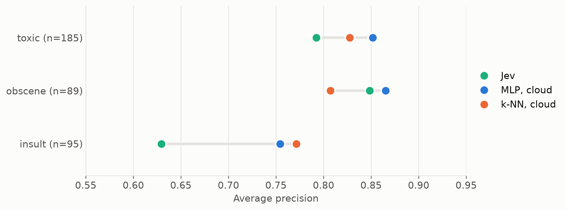 Figure 4: Average precision on the three labels with enough examples to measure. Jev is close to the custom models on
 obscene, but well behind on insult.
On obscene, Jev is roughly level with the custom models. Swear words and sexual language are easy to recognize without seeing any examples.
On insult, Jev falls clearly behind, for the same reason as in the threshold section, only stronger. Jev scored 112 comments at 0.9 or higher for insult that the raters didn't label as insults. Almost half of them, 51, are labeled toxic, and many are personal attacks by any reading: "Man, you are really a dishonest person, disgusting!!!!", or "How primitive are you Are you from a nursery school?" Meanwhile, Jev scored all but one of the 95 comments the raters did call insults above 0.5. The raters used insult for a narrower set of comments than my question describes, and the custom models learned that narrower definition from the labels.
That's a useful reminder of what a zero-shot model is measured against. When my definition and the dataset's agree, as with obscene, Jev comes close to models built from 8,000 labels. When they don't, I'd need to either rewrite the question to match the raters, or accept that Jev is answering a slightly different question.
The other three labels are too small to compare: with 20, 13 and 6 examples, a single comment moves the scores by several points.
How many labels does each approach need?
A model trained on 8,000 labels beating one trained on none isn't a fair fight. The real question for a project like my blog is what happens with fewer labels.
So I rebuilt the custom models from smaller random subsets of the labeled data, from 15 to 8,000 comments, ten times each. For Jev, the labels don't train anything, but they are still useful: they're what I use to pick the threshold. So for each budget, I picked Jev's threshold using that many labeled comments and measured F1 on the rest. The custom models use the default 0.5 threshold.
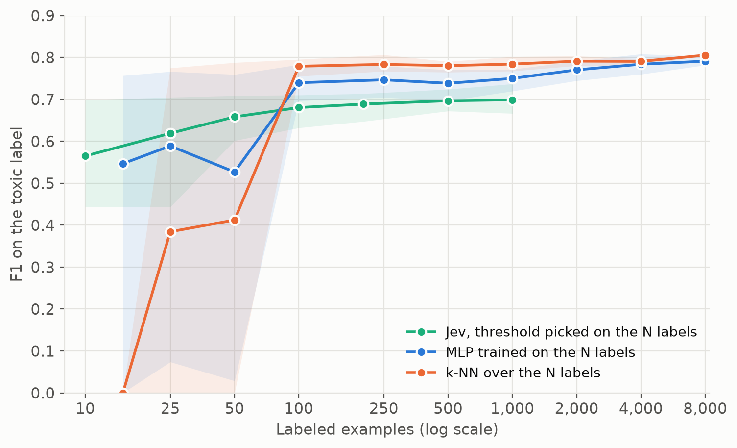 Figure 5:
 toxic F1 as the number of labeled comments grows, on a log scale. For Jev, the labels are only used to pick the threshold. For the MLP and k-NN, they are the training set. Shaded areas show the range between the 10th and 90th percentile across random subsets.
| Labeled comments | Toxic among them | Jev | MLP, cloud | k-NN, cloud |
|---|---|---|---|---|
| 25 | 1 to 8 | 0.62 | 0.59 | 0.38 |
| 50 | 1 to 9 | 0.66 | 0.53 | 0.41 |
| 100 | 7 to 15 | 0.68 | 0.74 | 0.78 |
| 1,000 | 86 to 116 | 0.70 | 0.75 | 0.78 |
| 8,000 | 786 | 0.79 | 0.81 |
Three things stand out:
- Jev is useful with almost no labels. With 50 labeled comments, it reaches 0.66 F1, and more labels barely help: picking the threshold from 1,000 labels only gets it to 0.70. With 25 or more labels, the chosen threshold almost always lands at 0.92 or 0.93.
- Below about 100 labels, the custom models are a gamble. With 25 or 50 labels, there are only a handful of toxic comments to learn from, and the result depends on which ones you happened to get. The shaded areas span almost the whole chart: some subsets give a decent model, others give one that never flags anything.
- With cloud embeddings, around 100 labels is enough to beat Jev on
toxic. That's about ten toxic examples. I expected the crossover to take thousands.
The k-NN line starts at zero for a reason I'll come back to below.
The toxic label is the easy case: 1 in 11 comments has it. For the rare labels, the training data simply doesn't contain enough examples. Averaged across all six labels, Jev's average precision is 0.53, and the custom models only catch up at around 2,000 labeled comments.
The embedding matters more than the classifier
So far I've focused on the cloud embeddings, because the MiniLM versions were never competitive. It's worth looking at how big the gap is.
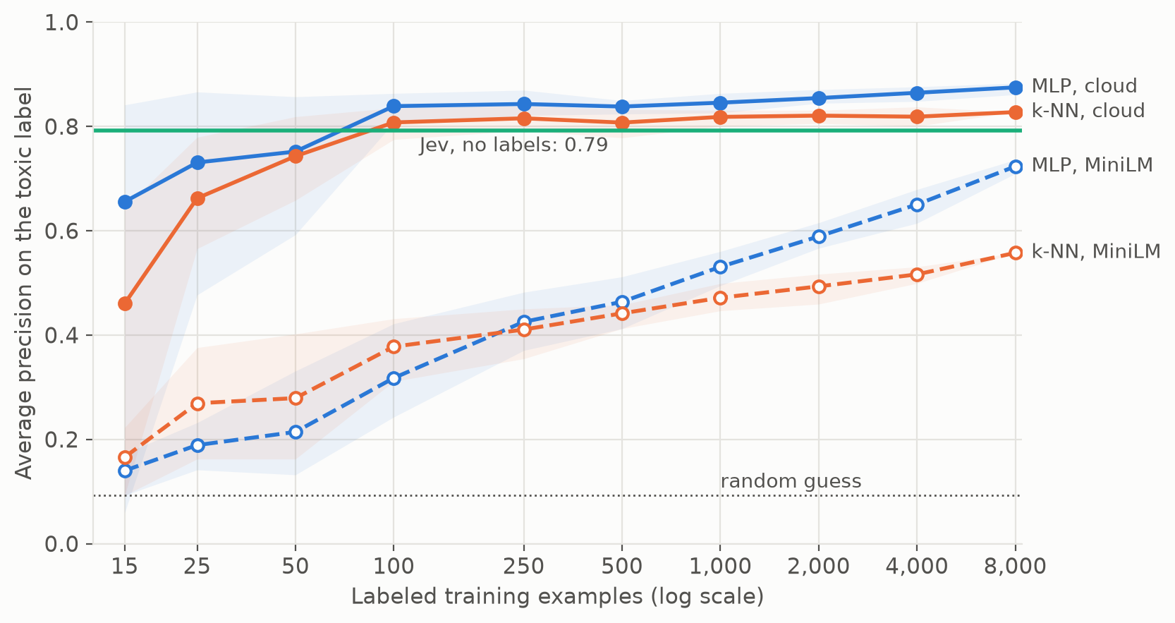 Figure 6: Average precision on the
 toxic label as the training set grows. Solid lines use cloud embeddings, dashed lines use MiniLM. 100 examples on cloud embeddings beat 8,000 on MiniLM.
The MLP trained on 100 cloud-embedded comments reaches 0.84 average precision. Trained on all 8,000 MiniLM-embedded comments, it reaches 0.72. Eighty times more training data doesn't make up for the weaker embeddings.
The choice of classifier matters much less. On cloud embeddings, the MLP and k-NN are close: k-NN has the better F1, the MLP the better average precision. On MiniLM, the MLP is clearly better than k-NN. A likely explanation is that k-NN treats every dimension of the embedding as equally important, so it finds comments about the same topic rather than comments with the same tone, while the MLP can learn which dimensions matter. I didn't test that directly.
MiniLM is a general-purpose model trained to group sentences by meaning. The cloud model was asked for embeddings meant for classification, and it's a much larger model. For a task that depends on tone more than topic, that difference dominates.
A closer look at k-NN
k-NN was the approach I expected least from, and it ended up being the most interesting. It doesn't train, so adding a labeled comment just means storing one more embedding, and every decision can be explained by showing the comments it was based on. Two questions decide how well it works: how many examples it needs, and how many neighbors it should look at.
The first answer depends on the number of positive examples, not the total number of labels. Grouping the runs from the previous section by how many toxic comments they happened to contain makes that clear:
| Toxic comments among the labels | toxic F1 | Average precision |
|---|---|---|
| 0 to 3 | 0.00 | 0.29 to 0.61 |
| 4 to 6 | 0.71 | 0.73 |
| 7 to 10 | 0.78 | 0.82 |
| 11 to 30 | 0.78 | 0.81 to 0.82 |
| 786 (all 8,000 labels) | 0.81 | 0.83 |
With 7 neighbors, a comment only scores 0.5 or higher if at least 4 of its neighbors are toxic, so with fewer than 4 toxic examples k-NN can't flag anything. That's why its line in Figure 5 starts at zero. Its ranking is already useful at that point, and fewer neighbors fix the problem: with only 2 or 3 toxic examples, looking at 3 neighbors gets 0.60 F1. From about 10 toxic examples on, k-NN with 7 neighbors is within a few points of where it ends up with all 786.
Which raises the second question. Seven neighbors made sense for a small dataset, but with 8,000 labels there's room for more. To choose without peeking at the evaluation comments, I scored every labeled comment using its nearest other labeled comments, and picked the number of neighbors that ranked them best. That was 51. On the evaluation comments:
| k-NN on cloud embeddings | ROC-AUC | Average precision | F1 with a fair threshold |
|---|---|---|---|
| 7 neighbors | 0.96 | 0.83 | 0.80 |
| 51 neighbors | 0.98 | 0.90 | 0.79 |
| For comparison: MLP | 0.96 | 0.85 | 0.77 |
With 51 neighbors, k-NN ranks toxic comments better than anything else in this comparison, and it beats the MLP's average precision in every bootstrap resample. It doesn't help where it counts for a yes/no decision, though: F1 stays the same, and so does the average across all six labels. For rare labels like threat, which has 27 examples in the whole training set, 51 neighbors mostly dilutes the few positives. The right number of neighbors grows with the number of positive examples, so it's something to revisit as the labels pile up, label by label.
The weaknesses are the ones you'd expect. k-NN is only as good as the embeddings: on MiniLM, it ends up as the weakest approach, and even 101 neighbors only lift its average precision to 0.65. And its cost grows with the data, since every comment is compared against every stored example. That's 13 ms for 8,000 comments, but a site with millions of labeled comments would need a vector index to keep it fast.
Speed, cost and trade-offs
Accuracy is only part of the decision. The approaches also differ in how fast they answer, what each comment costs, and how much work they take to set up and keep running.
Per comment
| Pipeline | Median time | Tokens per comment | Cost per 1,000 comments |
|---|---|---|---|
| MiniLM + MLP | 10 ms | none | none |
| MiniLM + k-NN | 12 ms | none | none |
| Cloud embeddings + MLP | 254 ms | about 80 | about $0.016 |
| Cloud embeddings + k-NN | 267 ms | about 80 | about $0.016 |
| Jev, all six questions | 209 ms | about 935 in, 111 out | about $0.039 |
Jev, toxic only | 206 ms | about 450 in, 21 out | about $0.019 |
I measured the local pipelines on my laptop's CPU, an AMD Ryzen 7 5800H. For the network calls, I sent 60 evaluation comments from the same laptop, one request at a time, alternating between the embedding API and Jev so that both saw the same network conditions. The costs use the prices listed today: Jev 1.13 charges $0.042 per million input tokens, and output tokens are free. Google's pricing page lists $0.20 per million tokens for its current embedding model; it doesn't list gemini-embedding-001 separately, so I used the same price.
A few things in that table surprised me:
- Jev was faster than the embedding call on its own. The median embedding request took 254 ms, against 209 ms for Jev answering all six questions. The cloud pipelines still have to run the classifier after that, so the trained model doesn't buy any speed over Jev unless the embedding model runs locally.
- More questions cost tokens, not time. Asking one question took about as long as asking six. Each extra question adds about 100 input tokens on top of a fixed cost of about 360 tokens per request, which includes the comment itself.
- The money is small for everyone. With all six questions, Jev costs about 4 cents per thousand comments. The embedding call costs about 1.6 cents. Only the local pipeline is free, and only because you're paying for the CPU yourself.
For this blog, none of this matters: comments arrive a few times a week, and moderation runs in the background after the comment is saved. At a million comments a day, it starts to: about $39 a day for Jev with six questions, $16 for the embedding calls, and nothing for MiniLM. Jev also has a default rate limit of 80 requests per second, which is about 7 million requests a day.
Setting it up and keeping it running
| Custom model, MiniLM | Custom model, cloud embeddings | Jev | |
|---|---|---|---|
| Labels to get started | Thousands, and it keeps improving | About 10 positives per label | None, about 50 to pick a threshold |
| One-time work | Embed the labels locally, then train the MLP (3 s) or store the embeddings | Embed the labels through the API, then train the MLP (7 s) or store the embeddings | Write the questions |
| What you host | A 91 MB embedding model plus the MLP or the stored embeddings | The MLP or the stored embeddings | Nothing |
| When the definition changes | Relabel, then retrain the MLP; k-NN only needs the new labels | Same | Edit the question, then check the threshold |
| When the model changes | Re-embed every labeled comment | Same | Check the threshold again |
| Where the comment goes | Nowhere: it can run in the browser | TypeSafe |
The biggest cost of a custom model isn't in either table: it's the labels. Training takes seconds and the API calls cost cents, but someone has to read and label every comment first. Even at five seconds a comment, the 8,000 labels in this dataset are 11 hours of work, and the rare labels need thousands of comments to collect enough examples.
The last row is the one that matters most for some sites. A MiniLM model can run entirely in the reader's browser, as I showed in the earlier post, so the comment never leaves their device. Both the cloud embeddings and Jev send the comment text to a third party.
What this doesn't tell you
- The rare labels are too small to judge.
threathas 6 examples in the evaluation set andidentity_hatehas 13. A single comment moves their scores a lot, so I've avoided drawing conclusions from them individually. - The labels are noisy. As the examples above show, some "false positives" are really labeling mistakes. Precision for every approach is measured against those labels, which hurts an approach that disagrees with the raters' habits more than one that learned them.
- I wrote one set of questions. I didn't iterate on the wording of Jev's questions, and I didn't tune the MLP beyond the setup from the earlier post. Both could probably do better.
- The cloud embedding model changed. My first PyTorch post used
text-embedding-004. This comparison usesgemini-embedding-001, so the cloud numbers aren't directly comparable with that post.
The code, cached predictions and analysis scripts are in the repository.
Conclusion
So, would a model trained on my own comments be more accurate than Jev? On this dataset, yes, if I had good embeddings and around a hundred labeled comments, as long as about ten of them are examples of what I'm looking for. That's far fewer than I expected.
But that comes with conditions. The embedding model has to suit the task, because the wrong one cost more accuracy than any other choice in this comparison. Every label needs its own handful of positive examples, which takes thousands of comments for the rare ones. And then there's the pipeline: embeddings, a stored dataset or a trained model, a threshold, and hosting. Of the two custom models, k-NN is the easier one to live with: there's no training step, and every new label improves it immediately.
Jev skips all of that. It ranked comments as well as the custom models by ROC-AUC, it was a little less precise at the top of the list, and it needed about 50 labeled comments to pick a threshold, not to learn the task. When the definition changes, I edit a sentence.
For this blog, where I have a hundred comments, one question, and no interest in maintaining a training pipeline, that's still the right trade. If I ever have thousands of labeled comments and a reason to care about the last few points of precision, I now know the custom model is worth building, and that the first thing to get right is the embedding model.
Comments
No comments yet. Be the first to comment!
Leave a comment
Comments are moderated and may take some time to appear.